Partial wavelet coherence
This script demonstrates how to do partial wavelet coherence using the WaveletCoherence class from nnsa. It first shows PWC with one confounding variable, and then PWC with 2 confounding variables.
Author: Tim Hermans (tim-hermans@hotmail.com).
Link to script: cwt/partial_wavelet_coherence.py
import numpy as np
import matplotlib.pyplot as plt

from nnsa import WaveletCoherence
from nnsa.utils.plotting import save_fig_as, scale_figsize

plt.close('all')
fig_width = 18
Settings.
# Data settings.
np.random.seed(43)
N = 1024
fs = 256
t = np.arange(N)/fs

# Wavelet settings.
cwt_kwargs = dict(
    wavelet='Morlet(6)',
    coimode='moi',
)

# Optional surrogate settings.
surrogates_kwargs = dict(
    how='AR',
    n_surrogates=0,
    seed=43,
)
Create test data.
# x and y.
f_all = [4, 8, 16, 32, 64]
a_all = np.array([1, 1, 1, 1, 1])
phi_all = np.array([-180, -90, 0, 90, 180])/180*np.pi
x = np.random.rand(N) - 0.5
y = np.random.rand(N) - 0.5
for a, f, phi in zip(a_all, f_all, phi_all):
    x += a * np.sin(t*2*np.pi*f + phi)
    y += a * np.sin(t*2*np.pi*f)

# Add a confounding signal z to x and y to 'overshadow' their true interaction.
z = np.cumsum(5*(np.random.rand(N)-0.5))
snr = 0.5
xz = snr*x + z + np.random.rand(N)
yz = snr*y + z + np.random.rand(N)
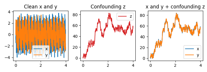
Plot signals.
fig, axes = plt.subplots(1, 3, tight_layout=True, sharex='all',
                         figsize=scale_figsize((10, 3.5), width=fig_width, unit='cm'),
                         )
axes[0].plot(t, x, label='x')
axes[0].plot(t, y, label='y')
axes[1].plot(t, z, color='C3', label='z')
axes[2].plot(t, xz, label='x')
axes[2].plot(t, yz, label='y')

axes[0].set_title('Clean x and y')
axes[0].legend()
axes[1].set_title('Confounding z')
axes[1].legend()
axes[2].set_title('x and y + confounding z')
axes[2].legend()
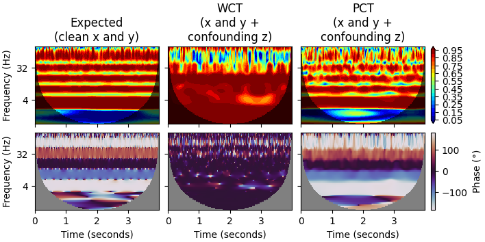
Compute (partial) wavelet coherence with one confounding variable.
# Init wavelet coherence object.
wcoh = WaveletCoherence(cwt_kwargs=cwt_kwargs,
                        surrogates=surrogates_kwargs)

# Wavelet coherence between original x and y (without confounding z).
exp_result = wcoh.wct(x, y, fs, labels=['x', 'y'])

# Wavelet coherence between disturbed x and y (by confounding z).
wct_result = wcoh.wct(xz, yz, fs, labels=['x', 'y'])

# Partial wavelet coherence between disturbed x and y, controlling for confounding z.
pct_result = wcoh.pct(xz, yz, z, fs, labels=['x', 'y', 'z'])
Plot wavelet results.
fig, axes = plt.subplots(2, 3, layout="constrained", sharex='all', sharey='all',
                         figsize=scale_figsize((10, 5), width=fig_width, unit='cm'),
                         )
exp_result.plot_scalogram(ax=axes[0, 0], add_colorbar=False)
exp_result.plot_phase(ax=axes[1, 0], add_colorbar=False, cmap='twilight', mask_non_significant=False)
wct_result.plot_scalogram(ax=axes[0, 1], add_colorbar=False)
wct_result.plot_phase(ax=axes[1, 1], add_colorbar=False, cmap='twilight', mask_non_significant=False)
pct_result.plot_scalogram(ax=axes[0, 2], add_colorbar=True)
pct_result.plot_phase(ax=axes[1, 2], add_colorbar=True, cmap='twilight', mask_non_significant=False)

for ax in np.reshape([axes[:, 1:]], -1):
    ax.set_ylabel('')
for ax in np.reshape([axes[:-1, :]], -1):
    ax.set_xlabel('')
for ax in axes[1, :]:
    ax.set_title('')

axes[0, 0].set_title('Expected\n(clean x and y)')
axes[0, 1].set_title('WCT\n(x and y +\nconfounding z)')
axes[0, 2].set_title('PCT\n(x and y +\nconfounding z)')
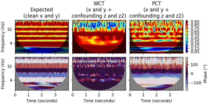
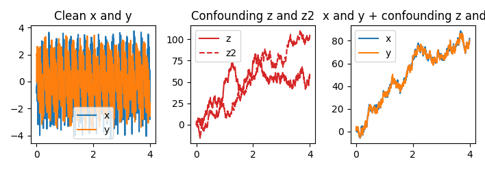
To compute partial wavelet coherence with two (or even more) confounding signals, we just use a list for the z argument in the pct() function.
# Create extra confounding signal.
z2 = np.cumsum(5*(np.random.rand(N)-0.5))
xz2 = snr*x + 0.5*(z + z2) + np.random.rand(N)
yz2 = snr*y + 0.5*(z + z2) + np.random.rand(N)
Plot signals.
fig, axes = plt.subplots(1, 3, tight_layout=True, sharex='all',
                         figsize=scale_figsize((10, 3.5), width=fig_width, unit='cm'),
                         )
axes[0].plot(t, x, label='x')
axes[0].plot(t, y, label='y')
axes[1].plot(t, z, color='C3', label='z')
axes[1].plot(t, z2, color='C3', ls='--', label='z2')
axes[2].plot(t, xz2, label='x')
axes[2].plot(t, yz2, label='y')

axes[0].set_title('Clean x and y')
axes[0].legend()
axes[1].set_title('Confounding z and z2')
axes[1].legend()
axes[2].set_title('x and y + confounding z and z2')
axes[2].legend()
Compute wavelet coherences.
# Compute regular wavelet coherence (WCT).
wct2_result = wcoh.wct(xz2, yz2, fs, labels=['xz', 'yz'])

# Compute partial wavelet coherence (PCT).
pct2_result = wcoh.pct(x=xz2, y=yz2, z=[z, z2], fs=fs, labels=['xz', 'yz', 'z', 'z2'])
Plot wavelet results.
fig, axes = plt.subplots(2, 3, layout="constrained", sharex='all', sharey='all',
                         figsize=scale_figsize((10, 5), width=fig_width, unit='cm'),
                         )
exp_result.plot_scalogram(ax=axes[0, 0], add_colorbar=False)
exp_result.plot_phase(ax=axes[1, 0], add_colorbar=False, cmap='twilight')
wct2_result.plot_scalogram(ax=axes[0, 1], add_colorbar=False)
wct2_result.plot_phase(ax=axes[1, 1], add_colorbar=False, cmap='twilight')
pct2_result.plot_scalogram(ax=axes[0, 2], add_colorbar=True)
pct2_result.plot_phase(ax=axes[1, 2], add_colorbar=True, cmap='twilight')

for ax in np.reshape([axes[:, 1:]], -1):
    ax.set_ylabel('')
for ax in np.reshape([axes[:-1, :]], -1):
    ax.set_xlabel('')
for ax in axes[1, :]:
    ax.set_title('')

axes[0, 0].set_title('Expected\n(clean x and y)')
axes[0, 1].set_title('WCT\n(x and y +\nconfounding z and z2)')
axes[0, 2].set_title('PCT\n(x and y +\nconfounding z and z2)')