Side obsp
This script demonstrates the use of SIgnal DEcomposition based on Obliques Subspace Projections (SIDE-ObSP) as proposed by Caicedo et al. This algorithm was proposed in the paper to decompose NIRS signals. This script demonstrates this algorithm by implementing the simulation study of the paper.
- References:
Caicedo et al., Decomposition of Near-Infrared Spectroscopy Signals Using Oblique Subspace Projections: Applications in Brain Hemodynamic Monitoring, Frontiers in Physiology (2016). https://doi.org/10.3389/fphys.2016.00515
Link to script: side_obsp.py
import matplotlib.pyplot as plt
import numpy as np
from scipy import signal

from nnsa import Butterworth, SideObsp
“We considered N = 1024 observations … following the model y = f1(x1) + f2(x2) + f3(x3) + eta, where eta is uniformly distributed random noise with zero mean, and a chosen standard deviation such that we obtain a signal-to-noise ratio SNR = 4db in the signal y.”
Define some settings.
# Number of samples.
N = 1024

# Signal to noise ratio in dB.
SNR_db = 4

# Convert dB to linear scale.
SNR = 10**(SNR_db / 10)  # Converting dB to linear scale

# Order of the moving average model in SIDE-ObSP (number of taps).
order = 50

# Seed the random generator.
np.random.seed(0)
“The function f1 was selected as a 3rd order low-pass Butterworth filter, with normalized frequency of 0.15 half-cycles/sample, the functions f2, and f3 had normalized frequencies of [0.1-0.2] half-cycles/sample and [0.05-0.15] half-cycles/sample, respectively.”
Create the butterworth filters which form the function f1, f2, f3. Here, we can make use of the Butterworth class of nnsa. We specify a sampling frequency of 2, so that the cut-off frequencies correspond to half cycles/sample. Judging from the figure with the impulse responses (figure 2), we need to switch the definitions for f2 and f3.
f1 = Butterworth(order=3, fn=0.15, filter_type='low', fs=2)
f2 = Butterworth(order=3, fn=[0.05, 0.15], filter_type='band', fs=2)
f3 = Butterworth(order=3, fn=[0.1, 0.2], filter_type='band', fs=2)

# Plot original impulse responses (figure 2 in the paper).
figsize = np.array((6, 4))
fig, axes = plt.subplots(3, 1, sharex='all', tight_layout=True, figsize=figsize)
axes = np.reshape([axes], -1)
imp = signal.unit_impulse(shape=order)
for ii, (f, ax) in enumerate(zip([f1, f2, f3], axes)):
    response = f.filter(imp)
    ax.plot(response, color='k', linestyle='--', label='Original')
    ax.set_ylabel(f'h{ii+1}')
    ax.grid(True)
    ax.legend()

axes[-1].set_xlabel('Samples')

“We considered the inputs {x1, x2, x3}, to be three binary pseudorandom signals (PBRN) in the normalized frequency range [0-0.3] half-cycles/sample.”
Create the simulation data. I don’t know exactly how the “binary pseudorandom signals (PBRN) in the normalized frequency range [0-0.3] half-cycles/sample” ought to be created, so instead I just create a random white noise signal and then filter it in the range [0-0.3] using a butterworth filter.
f0 = Butterworth(order=8, fn=0.3, filter_type='low', fs=2)

# Generate random signals
x1 = f0.filter(np.random.normal(0, 1, size=N))
x2 = f0.filter(np.random.normal(0, 1, size=N))
x3 = f0.filter(np.random.normal(0, 1, size=N))
x4 = f0.filter(np.random.normal(0, 1, size=N))
“In addition we induced a correlation of rho = 0.5 between the input signals by adding a 4th reference PBRN signal, x4, to all the inputs.”
Add correlation to inputs (equation 16).
def impose_corr(a, b, rho):
    return rho * b + np.sqrt(1 - rho ** 2) * a


x1 = impose_corr(x1, x4, 0.5)
x2 = impose_corr(x2, x4, 0.5)
x3 = impose_corr(x3, x4, 0.5)
“Before applying SIDE-ObSP, we also contaminated all the inputs with uniformly distributed random noise N(0, sigma), where sigma was chosen to reach a SNR = 4dB.”
Add noise.
def add_noise(x):
    # Generate uniformly distributed random noise.
    eta = np.random.uniform(-1, 1, len(x))

    # Adjust the noise to have zero mean and standard deviation such that provided SNR is achieved.
    eta -= np.mean(eta)
    eta /= np.std(eta)
    eta *= np.sqrt(np.sum(x**2) / len(x) / SNR)

    # Add noise.
    xn = x + eta

    return xn


x1 = add_noise(x1)
x2 = add_noise(x2)
x3 = add_noise(x3)
Create the mixed signal y.
fx1 = f1.filter(x1)
fx2 = f2.filter(x2)
fx3 = f3.filter(x3)
y = fx1 + fx2 + fx3

# Add noise.
y = add_noise(y)
“In addition, to complicate more the decomposition problem, we filtered the signal x4 using a low pass Buttherworth filter of 3rd order and normalized cut-off frequency of 0.3 half-cycles/sample, the filtered signal was mixed together with the output signal y, imposing a correlation of 0.3 between them, using Equation (16). “
f4 = Butterworth(order=3, fn=0.3, filter_type='low', fs=2)
x4 = f4.filter(x4)
y = impose_corr(y, x4, rho=0.3)
“We applied ObSP using the noisy inputs, xi and the noisy output y to find the linear contribution of each input on the output, yi = fi(xi).”
First, do SideObsp without regularization.
# Initiate SideObsp with required options.
so = SideObsp(
    # Order of the moving average model (number of taps).
    order=order,
    # Regulizer to use for the linear model.
    regularizer=None,
)

# Fit the model.
X = [x1, x2, x3]
so.fit(X, y)
Now, the impulse responses for each input are fitted and can be obtained by accessing the so.h attribute.
# Let's plot the fitted impulse reponses in the same figure as the orignal impulse responses (as in figure 2).
print('Shape of so.h:', so.h.shape)
for ii, (h, ax) in enumerate(zip(so.h.T, axes)):
    # We need to flip the impulse response to have it
    ax.plot(h[::-1], color='C0', label='Unregularized')
    ax.legend(loc='upper right')
Let’s use regularization to smooth the impulse response. Following the paper, we will find the regularization constants using 10-fold cross-validation (so we can leave gammas set to None).
so_smooth = SideObsp(order=50, regularizer='smooth', gammas=None)

# We need to find the hyperparameter gamma for each input. We can do this using fit_hyper(), which does a gridsearch.
# If we set gammas_all to None, a default list of gammas is tried (if gamma is not already defined).
so_smooth.fit_hyper(X, y, gammas_all=None, k_folds=10)

# With order and gammas defined, we can call the fit function to find the impulse responses.
so_smooth.fit(X, y)
Plot (figure 2).
for ii, (h, ax) in enumerate(zip(so_smooth.h.T, axes)):
    # We need to flip the impulse response to have it
    ax.plot(h[::-1], color='C2', label='Regularized')
    ax.legend(loc='upper right')

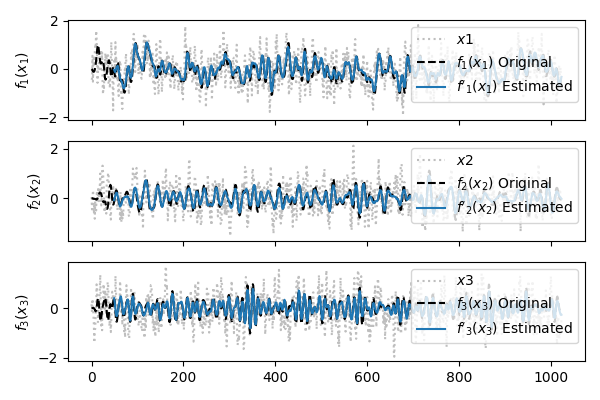
Once we fitted the model, we can estimate each input’s contribution to y. These should correspond to f1(x1), f2(x2) and f3(x3).
fX_pred = so_smooth.transform(X)

# Plot to compare estimated with true signal contributions.
fig, axes = plt.subplots(3, 1, tight_layout=True, sharex='all', figsize=figsize)
for ii, (ax, xi, fxi, fxi_pred) in enumerate(zip(axes, X, [fx1, fx2, fx3], fX_pred.T)):
    ax.plot(xi, color='C7', alpha=0.5, ls=':', label=f'$x{ii+1}$')
    ax.plot(fxi, color='k', ls='--', label=f'$f_{ii+1}(x_{ii+1})$ Original')
    ax.plot(fxi_pred, color='C0', label=f"$f'_{ii+1}(x_{ii+1})$ Estimated")
    ax.set_ylabel(f'$f_{ii+1}(x_{ii+1})$')
    ax.legend(loc='upper right')
If we expect that x3 is a source of noise for y, we can use SIDE-ObSP to denoise y with respect to x3.
# x3 was the third entry in X, so we extract the prediction of that one.
fx3_pred = fX_pred[:, 2]

# We can simply subtract the estimated (noisy) component due to x3 from y to denoise it.
y_min_fx3 = y - fx3_pred
We can do all of this in fewer lines of code, too. So, if the third input in X is expected to cause noise in y, we can separate the noise from the signal is just 2 lines of code:
# Estimate noise component (do gridsearch to find hyperparameters order and gammas).
x_noise = SideObsp(regularizer='smooth', order=None, gammas=None).fit_hyper(X, y).fit_transform(X, y, k=2)

# Denoise.
y_denoise = y - x_noise